Building Elbow Arrows in Excalidraw (Part 2)

In part one we identified the design goals (shortest route, minimal segments, proper arrow orientation and shape avoidance), but our naive and greedy first approach to the algorithm turned out to be inadequate on multiple fronts. Therefore this approach is abandoned in favor of a different algorithm.

Games to the Rescue

The design goals were suspiciously similar to the problem of pathfinding in video games, which is a common, well researched problem. Characters in these games often have to find their way from point A to point B on the game map, without getting blocked by obstacles and use the shortest route. They also need to make it look like a human would take that route, so these characters don’t break the immersion. Thus, we turn out focus to A* pathfinding.

Building the Foundations

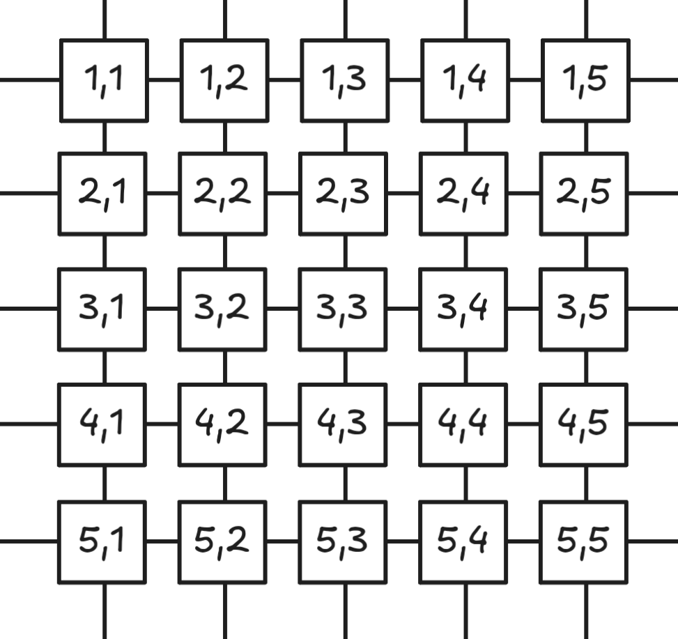
To understand A* pathfinding we need to understand the context, some of the other graph search algorithms it is built and improved on, and how can they help solve our challenge. To begin with, let’s talk about where A* comes from. It is part of a family of algorithms for graph search, which all aim to find the shortest path in a graph of nodes connected by edges. While this makes them useful far beyond just games, we’ll just focus on pathfinding in a 2D grid (i.e. the canvas). How do we convert the canvas into a graph you ask? If we split it up into a 2D grid (where at its extreme every pixel is its own cell), the neighboring (common) sides of each two cell can be represented by edges of a graph where the nodes such an edge connects are the cells themselves.

If we can find a route across these node edges (grid cells) satisfying our original constraints, we would just draw the elbow arrow itself!

Breadth-First Search

One simple graph search algorithm which finds the guaranteed shortest path in a graph is the humble Breadth-First Search (BFS), which is where we will start our exploration. In essence, BFS tries to visit all the directly connected unvisited nodes from already visited nodes in every iteration (with the start cell being the only visited node at the beginning), until the cell containing the end point is visited. While we do this exploration, we keep a record of which adjacent node we come from for every node as we visit them, forming a contiguous linked list back toward the start node. Then when we reach the end point cell (we can do an early exit, it will be optimal), we can backtrack through the linked list of edges all the way to the start. This will give us the shortest path, but it will not look like an elbow arrow and is definitely not visually pleasing. It is however a start we can build on!

NOTE: If you’re interested in diving deeper into BFS, DFS, and how A* works, I recommend this article, which dives deeper into these algorithms and offers interactive visualizations⁠. This article will only cover the key insights building toward the final elbow arrow implementation.

Dijkstra’s Algorithm

BFS creates the shortest path to our end cell, it also avoids obstacles, but it doesn’t look like an elbow arrow path. To have the right arrow shape (i.e. orthogonal bends), we need to find an incentive for our algorithm to take this desired path. This is where Dijkstra’s algorithm comes into play. This algorithm operates on weighted graph edges, using these weights as cost to visit a certain neighbor. To illustrate what this means to our 2D canvas grid, imagine that the canvas has a 3rd depth dimension. The cells along all the possible correct elbow arrow routes are flat, while everywhere else there is a steep height difference, creating a “wall”. Our “maze generator” can then take into account all remaining design goals and only create these valleys, which satisfy these requirements. Of course this “maze generator” cannot pre-compute the “terrain” because the grid (or graph) is infinite (Excalidraw has an infinite whiteboard canvas), so we need it to tell us at any cell which neighbors are cheap to visit and which are (preferably prohibitively) expensive.

Distance functions

The answer to our needs is a well chosen distance function of course! This way the edge weights should naturally decrease toward the end cell creating a downward “slope” on our terrain (a negative gradient), while hopefully make incorrect path choices expensive. When we talk distance we often refer to the Euclidean distance⁠ which is just the length of line segment connecting two endpoints, but there are some clever distance definitions which can help us out in this special maze generation.

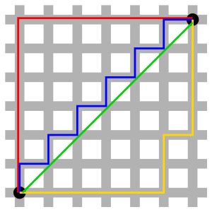
Our desired arrow route happens to be a Taxicab or Manhattan geometry⁠ and therefore we can use the Manhattan distance calculation to tell at every cell which neighboring cell takes us closer to our goal with it and get (some of) the right shape(s). This is calculated for two cells by first having the familiar Cartesian coordinates⁠ assigned to our 2D grid ([x = 12, y = -5] etc) and then adding together the absolute differences of their coordinates along each dimension. For example, if you have one point at [5, 12] and the other point at [10, -3] their Manhattan distance is |5 - 10| + |12 - (-3)| = 5 + 15 = 20. On the illustration below the green line is the Euclidean distance and the red, blue and yellow are equal Manhattan length paths.

Additional heuristics

Querying the Manhattan distance at every cell we want to visit in our Dijkstra Algorithm give us a metric we can use to generate the “maze” for our search algorithm, but it offers us multiple equally weighted paths and we need to choose the one with the shortest amount of orthogonal bends. So we add an additional term to our “maze generator” to not just consider the Manhattan distance of a neighboring cell and the end cell, but also increase the cost of neighbors if it would be a bend in the path, i.e. our search metric is: Manhattan distance + Bend count. This weighing function paired with Dijkstra’s Algorithm now generates correct, visually pleasing elbow arrows if there are no obstacles to avoid.

Exclusion Zones

In order to support shape avoidance we need to support the deactivation of some cells. These should behave like infinitely high walls in our maze, so the graph search algorithm never visits them. This is easily achieved by adding a flag to every cell and mapping shapes to these cells and disabling those cells the shapes cover. However combined with our modified distance calculation it starts to take sub-optimal paths around shapes. The reason is that we can’t see the entire “map” (i.e. the grid), it’s like a “fog of war” and we uncover it at every iteration of the search algorithm. Obstacles we should avoid well in advance might not be “seen” until it’s too late.

Of course introducing a backtracking process is one practical way to address this, but that can be computationally unfeasible. To reduce the unnecessary exploration steps and have a way to incorporate our heuristics, the A* algorithm seemed like an optimal choice. The A* algorithm is similar to Dijkstra’s Algorithm, it considers the weight of graph edges, but prioritizes exploring those neighboring nodes (or cells), which offer the best chance to take us closer to the end node (cell) and not waste precious computational cycles. It also promises a one-pass solution, which is also memory efficient.

What is A*?

The key insight of A* is that it balances two factors for every cell (node):

g(n): The actual cost to reach a node from the start. This will be our bend count and some additional heuristics later down the road
h(n): The estimated cost to reach the goal from that node (the Manhattan distance + grid exclusion + even more heuristic functions)
f(n) = g(n) + h(n): The total estimated cost of the path through that node

The algorithm maintains two sets of nodes:

Open set: Nodes to be evaluated
Closed set: Nodes already evaluated

The process:

Add the start node to the open set
Loop until the open set is empty:
- Select the node with the lowest f(n) score
- If it’s the goal, reconstruct the path and return
- Move it to the closed set
- For each neighbor:
- - Calculate tentative g score
  - If the neighbor is in the closed set and the new g score is worse, skip it
  - If the neighbor isn’t in the open set or the new g score is better:
  - - Update the neighbor’s scores
    - Set the current node as the neighbor’s parent
    - Add the neighbor to the open set
If the open set becomes empty without finding the goal, no path exists

By always exploring the node with the lowest f(n) value, A* efficiently finds optimal paths without exhaustively searching every possibility, which exactly what we want. At this stage the implementation mostly worked as expected, but edge cases kept popping up where a human would expect a different routing choice. The other problem was performance.

Performance Optimizations

While the behavior was close, the performance was really starting to cause problems, especially when multiple elbow arrow paths had to be calculated for every frame. Targeting at least 120Hz smooth rendering with ~50 elbow arrows re-routing every frame was a lofty, but achievable goal.

Binary Heap Optimization

The low hanging fruit was obviously the open set of nodes (cells). At every iteration a linear lookup across open nodes is not ideal. The obvious cure is a binary heap data structure with its O(log n) complexity.

Non-Uniform Grid

Operating on a pixel grid (or one node per pixel when looking at it as a graph) makes a significant amount of unnecessary A* iterations (99% and up, depending on conditions), which is a huge waste. Even having cells with just a few pixels is an unimaginable waste (and also wouldn’t be pixel perfect).

The solution to this problem is to draw a new grid, which only has nodes on a grid where a potential bend could be. Turns out this is easier than one would think, since aesthetically pleasing elbow arrows always break at shape corners, start and end point headings, and halfway between shapes to be avoided - with optional padding around shapes accounted for.

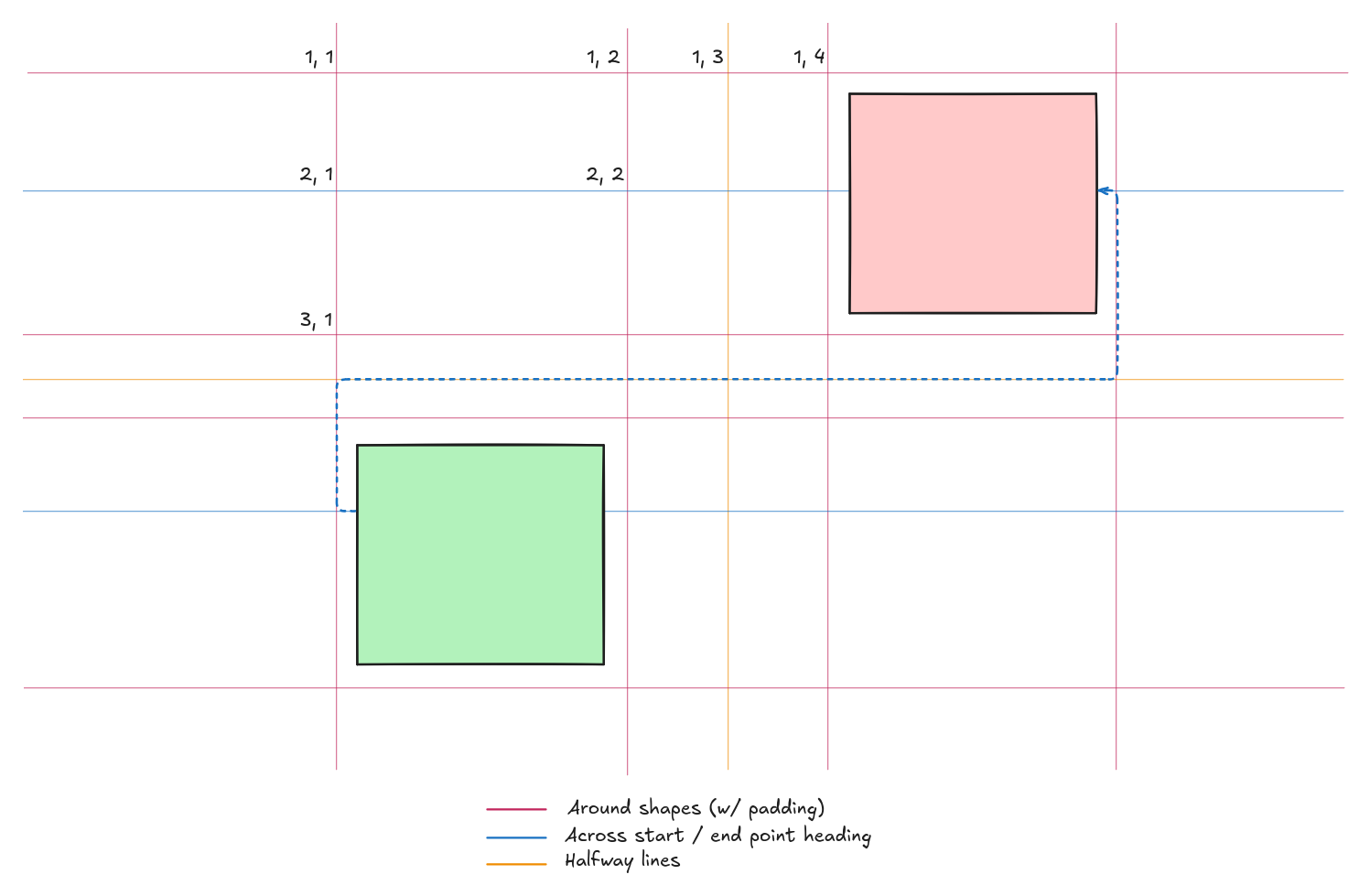
Since the algorithm operates on graph nodes, nothing forces us to make this a uniformly-sized grid (i.e. for the cells to be exactly the same size). The only thing that matters to A\* and the Manhattan distance calculation is neighboring cells and contiguous Cartesian coordinates. Lucky us!

Adapting A* with Manhattan distances for Aesthetic and Performant Elbow Arrows

Aesthetic Heuristics

While the basic A* implementation produced better results than the BFS approach, as mentioned previously, there were some cases beyond the excessive bend count that generated unnatural routes. With carefully constructing additional heuristics, we were able to address these, albeit changes to the A* metric unilaterally affect the behavior in all edge cases, so testing and fine-tuning happened manually to arrive at the final solution.

1. Backward Visit Prevention

Arrow segments are prohibited from moving “backwards,” overlapping with previous segments when there is no route other than backwards. This not just prevents spike-like paths (directly reversed segments), but almost completely avoids routes where a U-like arrow configuration would be required to avoid a shape.

This is achieved by tracking the direction of visits and looking back one step and forward one step to recognize the problematic configuration. Together with the very specific grid selection, this prevents the edge cases where this issue would trigger.

NOTE: This only works because there can be at most 2 closed axis-aligned bounding boxes (the shapes) to avoid. With more obstacles in between would certainly re-surface this issue.

2. Segment Length Consideration

Longer (Euclidean distance-wise) straight segments are preferred over multiple short segments, even though previously the Manhattan distance was selected as our main metric driving the A* pathfinding. This is because - again - in some edge cases the non-uniform grid would assume that what it generated was the shortest path, but when projected onto the pixel grid it clearly created short step patterns where it shouldn’t. It was especially prevalent with connected shapes being distant from each other.

3. Shape Side Awareness

When choosing between routing left or right around an obstacle, the algorithm considers:

The length of the obstacle’s sides
The relative position of start and end points heading-wise (see heading in part 1 of this series)
The parallel or orthogonal relation of the arrow and the shape’s bounding box side

4. Short Arrow Handling

Special logic for when the start and end points are very, very close, which prevents excessive meandering and loops. In one case where connected shapes almost overlap and the start and end points are very close, there is a hard-coded simplified direct route because the expected route would never emerge from the algorithm.

5. Overlap Management

The implementation also explicitly detects when shapes cover the start and/or end points. When connected shapes or points overlap, it selectively disables avoidance for one shape or both so there is a valid route possible, even if the exclusion zones would prevent it.

Conclusion

What started as a simple feature request - “add elbow arrows” - evolved into a sophisticated pathfinding challenge. By combining classical algorithms (A*), domain-specific optimizations (non-uniform grids, only two shapes to avoid etc.), and carefully tuned heuristics (aesthetic weights), Excalidraw’s elbow arrows speed up diagramming significantly and avoid diagrams previously hand-drawn and hand-managed.

It even made possible some other powerful features like keyboard shortcut flowchart creation⁠ which further empower Excalidraw users with serious diagramming needs.

Come join me for the 3rd and final part of this series on elbow arrows, where I walk you through how controlling and fixing arrow segments makes difficult-to-predict arrow routes possible for power users!